AN-20
Beginner’s Guide to PAD Power
Rev. C
Synopsis: The article provides a step by step guide for beginners using the PAD Power spread sheet, based on Excel, for analyzing power amplifier application circuits for reliability in terms of output transistor junction temperature and heat sink temperature. Some knowledge of the Excel spread sheet is assumed.
he safe operating area (SOA) of a power amplifier is its single most important specification. SOA graphs serve as a first approximation to help you decide if a particular power amplifier will meet the demands of your application. But a more accurate determination can be reached by making use of the PAD Power ™ spreadsheet that can be downloaded from the website. Consider the SOA graph below.
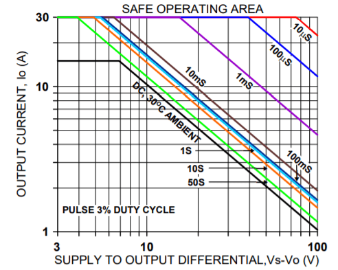
While the graph above adequately shows DC SOA and some pulse information it does not take into account ambient temperatures higher than 30°C, AC sine, phase or non-symmetric conditions that often appear in real-world applications. The PAD Power ™ spreadsheet takes all of these effects into account.
Step by Step Guide
Download and open the PAD Power spread sheet using the link provided above. At the bottom of the spreadsheet you will notice several page tabs. Click on “Readme” and study the introductory information on this page. We will expand upon the information in this article and add other details and tips as well.
Now click on the “Sine” page tab. You will notice a number of light-blue cells. These cells are for defining your application’s conditions for temperature, frequency and load. The spread sheet automatically recalculates results as you change operating conditions. You may find red pop-up information as you vary the input conditions. The information in red provides cautionary information or alerts you to dangerous conditions that need to be addressed. Don’t be concerned with the red warnings until all of your information is entered.
At cell E2 you may define the maximum junction temperature for the output transistors. A good rule of thumb is to set this number at 25°C less than the maximum junction temperature listed for the amplifier model used. Maximum junction temperature can be found in the specifications page for the amplifier model data sheet. Lower junction temperatures result in more reliable (longer life) application circuits and provide some margin in case some of the conditions specified later need to be estimated. In cell E2 type “150”.
Cell J2 defines the maximum ambient temperature expected. The amplifier needs clear open space around its heat sink to exhaust the hot air that is expelled by the amplifier’s cooling fan. This temperature may be higher than the temperature of the air going into the fan. Overall the “ambient” around the amplifier’s heat sink will be determined by the distance to various obstacles to free air flow around the amplifier, the power dissipation of the entire application circuit or system and how well the hot air is expelled from the system. At this stage of the analysis you may just have to estimate the temperature. At cell J2 type “30”.
Cell B4 defines the amplifier model. Click on this cell and you will find a pop-down menu with various amplifier models listed. For this example choose “PAD117”.
At cell E4 you will find another pop-down menu. Listed here are several common power amplifier application circuit configurations. For this simple example choose “Single Amp”. Whatever number is in cell G4 will be ignored when “Single Amp” is chosen.
Cells D6 and D7 define the power supply voltages. Note that amplifiers need some “head room”. That is to say, the power supply voltage needs to be higher than the expected output voltage peak. The amount of head room varies with the amplifier model and the peak output current. Refer to the product’s data sheet to find out what head room is needed for the expected peak output current and set the power supply accordingly. The specification of interest is “OUTPUT SWING”. Also consult the graph of typical output swing found in the “TYPICAL PERFORMANCE GRAPHS” pages of the data sheet. You also need to add the voltage drop in the connecting wires at the peak output current. It is usually not good practice to set the power supply voltage higher than needed because the excess voltage causes excess power dissipation in the amplifier which may limit the amplifier’s usefulness in the application and is wasteful of energy as well. In cell D6 enter “48” and in cell D7 enter “-48”. Needless to say the sum of these two numbers must be less than the maximum power supply voltage rating of the amplifier chosen. In this case the PAD117 is rated for 100V and the sum of the absolute values in cells D6 and D7 is 96V so this meets the requirement.
The next few light-blue cells define the signal expected at the load. At cell E10 select “Voltage” from the pop-down menu. This means that the intent of the application circuit is to control the voltage across the load. This is probably the most common application where some input voltage is amplified by some gain and the output voltage drives the load. At cell E11 type “90” and at cell I11 select “p-p” from the drop down menu. At cell H12 enter “0”. So far the output signal has been defined as a sine wave 90V p-p centered about 0 volts.
To further define the output signal enter at cell E13 “120” and at cell F13 enter “Hz” from the drop-down menu. At H13 enter “1” and at cell I13 enter “KHz” from the drop-down menu. At cell C15 click on “Continuous” from the drop-down menu. Altogether the output signal has been defined as a continuous 120 Hz to 1 kHz 90V p-p sine wave centered about 0V. Cells G15 and G16 will be ignored since “Continuous” was chosen at cell C15.
At cell E9 two types of analyses are offered: “use my input” and “find worst case”. Choose “find worst case”. When this option of chosen the input signal previously defined is interpreted as the maximum signal expected at the load and the temperatures calculated for junction and heat sink are the worst case expected as the signal across the load varies in amplitude, frequency and phase. More on this later.
The next few light-blue cells define the load conditions. For this example we will assume the PAD117 is driving a motor. The motor must be modeled as some inductance in series with some resistance. At cell B20 select “ohms=” from the drop-down menu and at cell C20 enter “10”. At cell B24 select “mH” from the drop-down menu and at cell C24 enter “3.3”. The motor is thus defined as 3.3mH of inductance in series with 10 ohms.
We will ignore lines 36 and greater for this example since these lines have to do with defining the load as some capacitance and resistance. Any red comments in this area can be ignored for this example.
At this point the amplifier model has been defined, its power supply voltages are set, and the output signal and load characteristics are defined. And we have chosen the “find worst case” analysis option.
Now it’s time to examine the results. To the right of the light-blue cells in the Load Definition section of the spread sheet you will find a number of cells in dark-blue. This area, ranging from cell D20 through G25, display the results
of calculations made for the lower frequency entered in cell E13. In these cells you can find “Vrms”, the rms voltage across the load, “Arms”, the rms current in the load, and “Wrms”, the power the load is dissipating. Similar results for
the higher frequency entered at cell H13 are displayed in the green cells H20 to K25.
More to the point of this exercise are the results displayed in dark-blue at cells F29 to F31. The results in these cells demonstrate one of the powerful features of PAD Power, namely, the “find worst case” analysis option chosen at cell
E9. As the output signal amplitude and frequency vary the power dissipation in the amplifier varies as well due to the changing amplitude and phase relationship of the output current and voltage. Based on the input conditions
given for maximum signal swing, power supply voltages and load conditions PAD Power calculates the worst case transistor junction temperatures and heat sink temperature (remember that the defined signal is interpreted as maximum when the “find worst case” analysis option is chosen). The results in these cells tell you if the amplifier will be overloaded anywhere in the operating range or not. The results listed for this example or well within the limits of the
PAD117 and this application, as defined, will be quite reliable.
The PAD117 is a rail to rail operational amplifier. This means that it works equally well with the input pins biased to either supply rail or at any voltage in between. The output, even at high currents, also approaches the power supply
voltages. The most common application utilizing this function is the single supply voltage amplifier where the +IN pin and the –Vs supply pin are grounded.
PAD Power can help with the analysis of a single power supply application as well. At cell D7 enter “0” and at cell D6 enter “48”. The application is now specified as a single supply of 50V (cell D6) and ground (0 volts) is specified for the negative supply voltage.
Since the output signal cannot be negative, because there is no negative supply voltage, the output signal must be re-specified. The previous specification was an output signal of 48V p-p and a frequency range of 120
Hz to 1 kHz. Let’s leave that specification as is. But the center point of the output needs to be shifted from 0 volts to half of the p-p value. At cell H12 enter “24”. The output signal is now specified as 48V p-p centered about 24V.
The output signal now has an “offset” of 24V. An analysis consequence of the offset is that the spread sheet will no longer automatically find the worst case temperatures. At cell E9 the analysis option “use my input” must be chosen.
The temperature calculation results shown in cells F29-F31 and cells J29-31 now reflect the defined signal but not necessarily the worst case temperatures as the signal amplitude and frequency vary. The temperatures displayed are
largely determined by the DC offset and won’t vary much with the AC amplitude entered at cell E11. The user can manually adjust the signal and observe how the temperatures vary. Several signal amplitudes and offsets (if
the offset varies) should be tried out and the resulting temperatures examined before the application can be determined as safe.
In this example you will note that the temperatures for the lower frequency (cells F29-31) are significantly different from the temperatures for the higher frequency (cells J29-31). This is due to the effect of phase difference between the output voltage and current at the high and low frequencies entered at cells E13 and H13.
It would appear that either of these applications with a frequency range of 120Hz to 1 kHz is good to go. Now that you are familiar with manipulating the input data for your application and you have seen how to interpret the
results you should be ready for more complex analysis. Notice that there are more page tabs at the bottom the spread sheet. These sheets cover piecewise linear analysis for output signals of non-repetitive signals and also a page to
help you with setting current limit for the various amplifier models using both standard and fold-over current limit. Explore these pages as you become more familiar with PAD Power.